The mechanical damage tool

Background

In recent years, much attention has focused on the issue of managing indoor climate in museums, libraries and archives in a responsible manner, especially in terms of reducing energy use and carbon emissions, but at the same time maintaining high standards of collection care.

The most general result of the scientific research into preventive conservation practice has been increasing skepticism regarding the concept of strict control of the museum climate. This has led to more relaxed specifications: individual long-term targets for specific collections, seasonal changes, and broader ranges of short-term fluctuations. This new understanding of collection requirements has been summarized in the IIC-ICOM CC Declaration of Environmental Guidelines in 2014 [ref. 1]:

For many classes of object[s] containing hygroscopic material (such as canvas paintings, textiles, ethnographic objects or animal glue) a stable relative humidity (RH) is required in the range of 40–60% and a stable temperature in the range 16–25°C with fluctuations of no more than ±10% RH per 24 hours within this range. More sensitive objects will require specific and tighter RH control, depending on the materials, condition, and history of the work of art. A conservator’s evaluation is essential in establishing the appropriate environmental conditions for works of art requested for loan.

These general specifications for climate are intended as a starting point and should be tailored to specific requirements of a specific object according to its material, construction and condition. Physical damage from climatic variations occurs when moisture-induced dimensional change of object’s component is restrained by another stronger component, and the restrained dimensional change exceeds a certain critical level. Therefore, decision makers in the heritage field need to know the quantitative interrelation between the intensity of the hazard (climate fluctuations), the direct cause of damage (dimensional response) and the risk of actual damage (the critical level of the restrained dimensional response bringing failure).

The mechanical damage tool is a software transforming climate versus time histories into dimensional change (strain) histories for a quantitative assessment of climate-induced risk of physical damage for various categories of cultural heritage objects:

• you upload one-year (or multiyear) temperature and relative humidity data which can be measured or simulated,
• you define the type and characteristics of the object,
• the software calculates the strain versus time history of the object exposed to the climate conditions introduced, 
• you select failure criteria to obtain risk indices for the specific object and climate.

The tool is simple-to-use and provides accurate ‘real-time’ moisture movement and the resulting strain experienced by the object in response to climatic variations.

1. J. Bickersteth, IIC and ICOM-CC Declaration on environmental guidelines. Studies in Conservation, 61sup1:12-7, 2016.

How the tool works - wooden panels

Step 1 - decomposition of relative humidity (RH) data

Yearly RH variations are a combination of long-term seasonal cycles, caused for example by an RH decrease in winter due to heating and a return to a higher RH level in summer, and irregular medium- and short-term changes arising from weather changes outside, the opening and closing of doors and windows, the flow of visitors, or the intermittent operation of climate control systems.

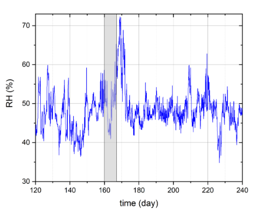
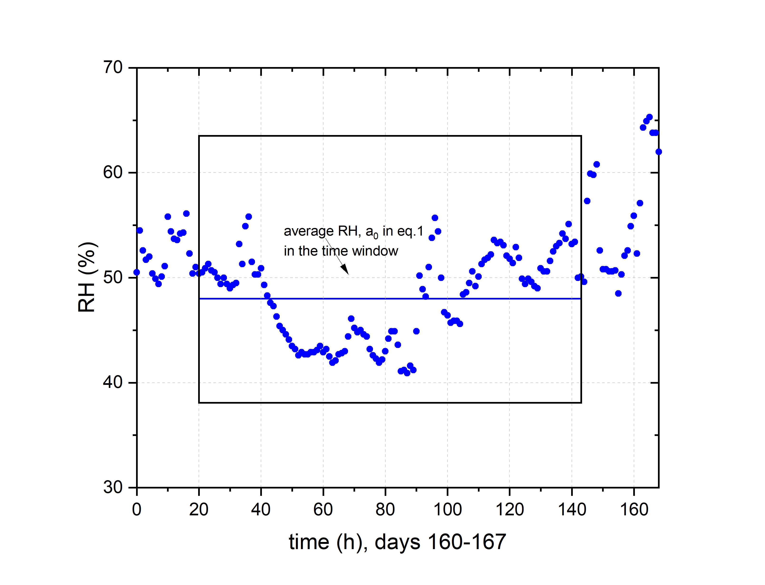
In the first step of the algorithm, the yearly or multi-year RH data (the climate history) is divided into smaller segments of equal length, the time windows. The RH data within each window are decomposed into a set of elementary RH cosine cycles of varying amplitude and duration using the discrete Fourier transform:

where \(a_0 \) is a constant corresponding to the average RH in the time window analysed, and \(a_i \), \( T_i\) and \( \phi_i \) determine amplitude, period and phase shift for each of the RH cosines, respectively. Therefore the constant \(a_0 \) determines the RH level around which the sum of the RH cosines (from here termed elementary RH cosines) oscillates. In the calculation procedure adopted, a 50% overlap of the time windows was used to mitigate potential problems at the window edges.

The length of the time window depends on the response time of a wooden panel. This response time is defined as the time needed to reach 63.2% (1-1/e) of the new equilibrium moisture content by wood for a given panel thickness, configuration of water vapour transport and temperature in response to a step change in RH. Water vapour transport can proceed through both the faces of a panel or through only one of the two faces – the coated face simulates the effect of a decorative layer completely blocking moisture flow through the top side. The response times of panels increase with increasing panel thickness, decreasing temperature (slower water vapour transport) or water vapour transport through one face only. The longer the response time, the greater the length of the time window. Based on an optimization procedure, the time window length is set in the software to be 8 times the response time of a panel.

The procedure is illustrated in the figures below:

Indoor RH in a museum gallery between May and September, data recorded at time intervals of 1 hour (top). A failure of climate control in June caused a short-term, abrupt increase in RH from the average of 45% to above 70%. Data for seven days (grey area) are shown in more detail (bottom). The discrete Fourier transform is performed on the data contained in the time window. An optimal window length of 123 hours, is used for the analysis of the response of a 10 mm thick wooden panel open to a water vapour flow through both faces as an example.

Step 2 – translating elementary RH cosines into elementary strain cosines in wooden panels

The pre-calculated elementary strain cosine database constitutes the core of the tool. The elementary strain cosines were obtained for the set of elementary RH cosines centred at 50% RH which is the mid-point of the full RH scale between 0 and 100%.

Each RH cosine of a given amplitude and period causes two consecutive swelling and shrinkage strains in a panel, the amplitude of which depends on the panel thickness, temperature and configuration of water vapour transport. The cycles of total strain experienced by a wooden panel subjected to elementary RH cosines were calculated with the use of finite element numerical simulations of water vapour transport and the moisture-related strain.

The simulation took into account two kinds of panels of varying thicknesses - freely-responding panels covered with a gesso layer (imitating panel paintings) and fully-restrained panels (imitating elements of wooden constructions). The panel, for which the elementary strain cycles should be obtained, is selected and defined by the user who can select between three wood species frequently used by artists, lime (linden), oak and poplar, two gesso formulations differing in stiffness, and two extreme ways in which the boards were cut out of the tree trunk, radial or tangential. The specific parameters for wood and ground layers used to model moisture transport and strain are detailed in the " Parameters for wood and ground layers " section.

The total strain is a sum of hygric strain, resulting from wood’s moisture-induced dimensional change, and elastic strain. Elastic strain is engendered by stresses which may result from all sources of restraint: external, moisture gradients across wood or mismatch in the moisture response of wood (strong) and the gesso layer (negligible). The average elastic strain over the entire thickness of a panel is used to assess risk of mechanical damage of wooden restrained panels. The elastic strain at the interface between the gesso layer and the wood substrate is used to assess risk of mechanical damage of a gesso layer laid on freely responding wooden panels .

As wooden panels are usually much longer and wider than they are thick, only moisture transport in the direction perpendicular to panel faces was considered, either radial or tangential, depending on how the panel was cut with respect to the anatomical direction of wood. As wood is non-responsive to moisture in the longitudinal direction, this direction was not included in the model.

The cycle of total strain experienced by a panel subjected to a specific elementary RH cosine is approximated by a cosine function, from here termed an elementary strain cosine, of the form:

where \( y_i \) is strain around which given elementary strain cosine oscillates, \( A_i \) [-] is its amplitude and \( \Delta t \) is a phase shift between RH and strain cosines. The amplitude of each elementary strain cosine is determined as half difference between the maximum and minimum strain values and \( y_i \) is set at this midpoint.

Strain induced at 21^oC by sinusoidal RH variations of ± 5% centred at 50% in a 20 mm, tangentially-cut wooden panel open to a water vapour flow through both faces. \(y_i \) and \( \Delta t \) parameters of Eq. 2, as well as the derived cosine function from the strain data, are indicated.

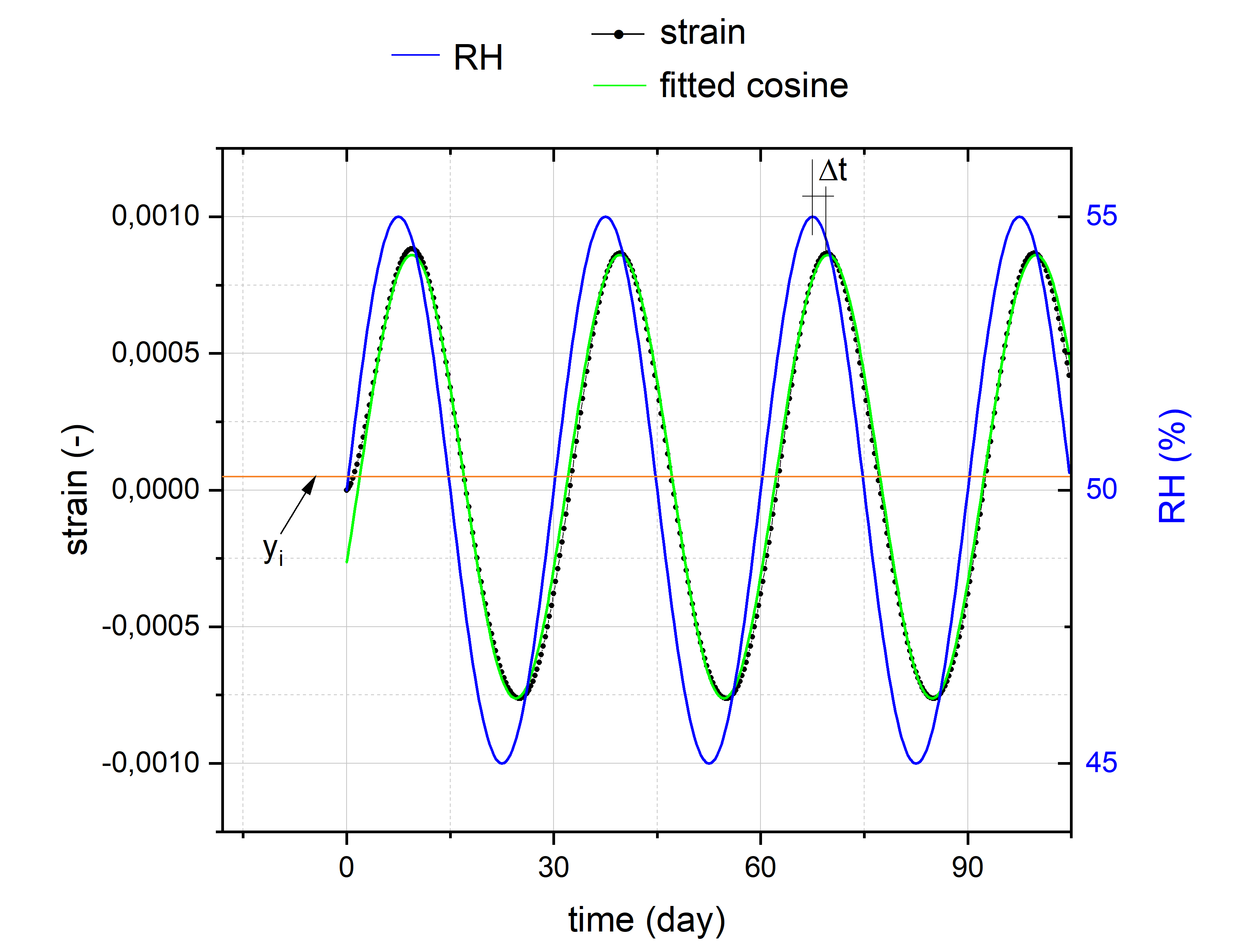
The database of elementary strain cosines was calculated for elementary cosine RH variations of selected amplitudes: 0.01, 0.1, 0.5, 1, 2, 5 and 10% RH. Fourier transforms performed on a variety of microclimates measured in museums or historical buildings with different long and short-term RH variations have shown that the RH amplitudes which come from the Fourier decomposition are rarely larger than 5%. However, in the unlikely case where the data processing tool identifies an elementary RH cosine of amplitude exceeding 10% in the Fourier transfer, the procedure is deemed to lose its reliability and is stopped. The selected cosine periods for elementary RH variations used to calculate the database were 0.04, 0.25, 0.5, 1, 4, 7, 30, 90 and 365 days which covers the whole range of time intervals present in typical RH histories of indoor climates in museums and historic buildings. Calculations were performed for combinations of four panel thicknesses (5, 10, 20 and 40 mm), two configurations of water vapour transport and four temperatures of 7, 15, 21 and 25 ^oC, so the database of elementary strain cosines contains 32 sets of functions. Interpolation is used when necessary to derive elementary cosines for a specific amplitude or period.

Step 3 - superposition of elementary strain cycles when zero strain is assumed at 50% RH (the mid-point of the full RH scale between 0 and 100%)

The elementary strain cosines in the softwaer database are pre-calculated for sinusoidal elementary RH cycles centred at 50% RH. It is assumed in the calculations that no forces (tensile or compressive) are present in the object at this RH level, and consequently no strains are experienced by any part of the object. From here, this RH level is termed the zero-strain RH level, to which the object has perfectly acclimatized.

In this step, the full strain history of an object, which is a dimensional response to the climatic variations analyzed in a given time window, is obtained by summing the elementary strain cycles corresponding to the elementary RH cycles obtained in step 1.

Using the elementary strain cosines, the RH series described by Eq. 1 is translated into a strain series of the form:

if the average RH or \( a_0 \) in Eq. 1 is 50% at which the strain was assumed to be zero.

As signaled in the description of step 2 above, the elementary strain cycles in the software database were calculated for four temperatures. Increasing temperature leads to an increase in the water vapour diffusion coefficient and faster movement of moisture across the material, but also to a decrease in water vapour sorption at a given RH. Using interpolation, the elementary strain cycles can be scaled to any temperature value selected. To make the simulation manageable, the elementary strain cycles used in the superposition procedure are calculated for a constant temperature defined as the long-term mean temperature determined from the climate data uploaded by the user. The value will be displayed by the software. We have verified that this simplified procedure satisfactorily accounts for temperature effects.

However, the strain series described by Eq. 3 requires a modification to represent the strain versus time history of a panel at an \( a_0 \) different from 50% due to the non-linear relationships between ambient RH and moisture content in wood, water vapour permeability and wood’s tensile properties, which all affect the moisture-related strain. Therefore, a scaling factor \( s_i (a_0,T_i) \) for the amplitude \(A_i(a_i,T_i) \) is introduced:

where \(\varepsilon_0(a_0)\) represents an overall dimensional change of a panel (shrinking or swelling) resulting from the change in the average RH from 50% to another specific value.

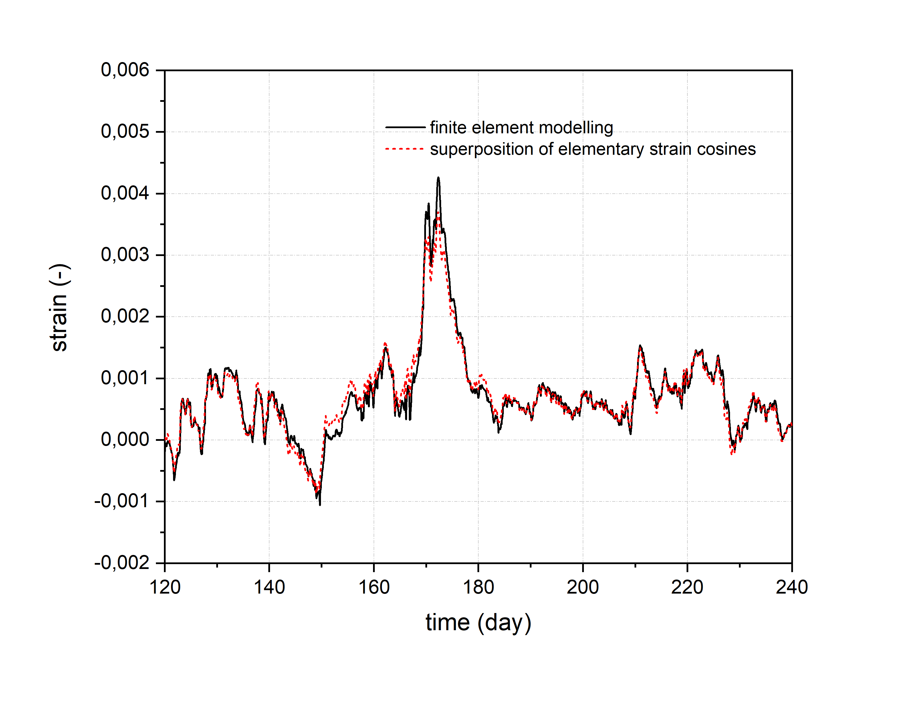
It has been verified that the superposition of the elementary strain cycles performed by the software is in agreement with the result of the full finite element numerical simulation for the object (see figure below).

Strain induced at 21 ^oC by RH variations in a museum gallery between May and September (shown above) for a tangentially-cut wooden panel open to water vapour flow through both faces

Step 4 – strain versus time histories when zero strain is assumed at an RH different from 50%

Heritage objects undergo strain patterns which can be complex when the RH departs from the zero-strain level at which no forces are present in the object. For example, a wooden panel covered with a layer of gesso may experience an uneven dimensional response in opposite faces of a panel owing to the differences in moisture-related dimensional response between wood and gesso. The stress induced by the uneven response will manifest in a cupping of the panel.

The software performs two operations to re-scale strain versus time histories and account for a shift of the zero-strain RH level from 50% to another RH level. This level can be a long-term average of the climate analyzed or a value selected by the user, for example the historic long-term average RH for which the zero-strain state (acclimatization) of the objects is assumed. First, the entire strain history is shifted by a certain value of strain so that the zero strain in the history corresponds to the RH level at which full acclimatization of the object is assumed. The strain values by which strain histories need to be shifted are pre-calculated in the database for systematically varied RH levels.

The strain history experienced by a 0.4 mm thick gesso layer laid on a 10 mm wooden panel open to water vapour flow through both faces is shifted when the assumed zero-strain RH level is changed from 50% to 60%.

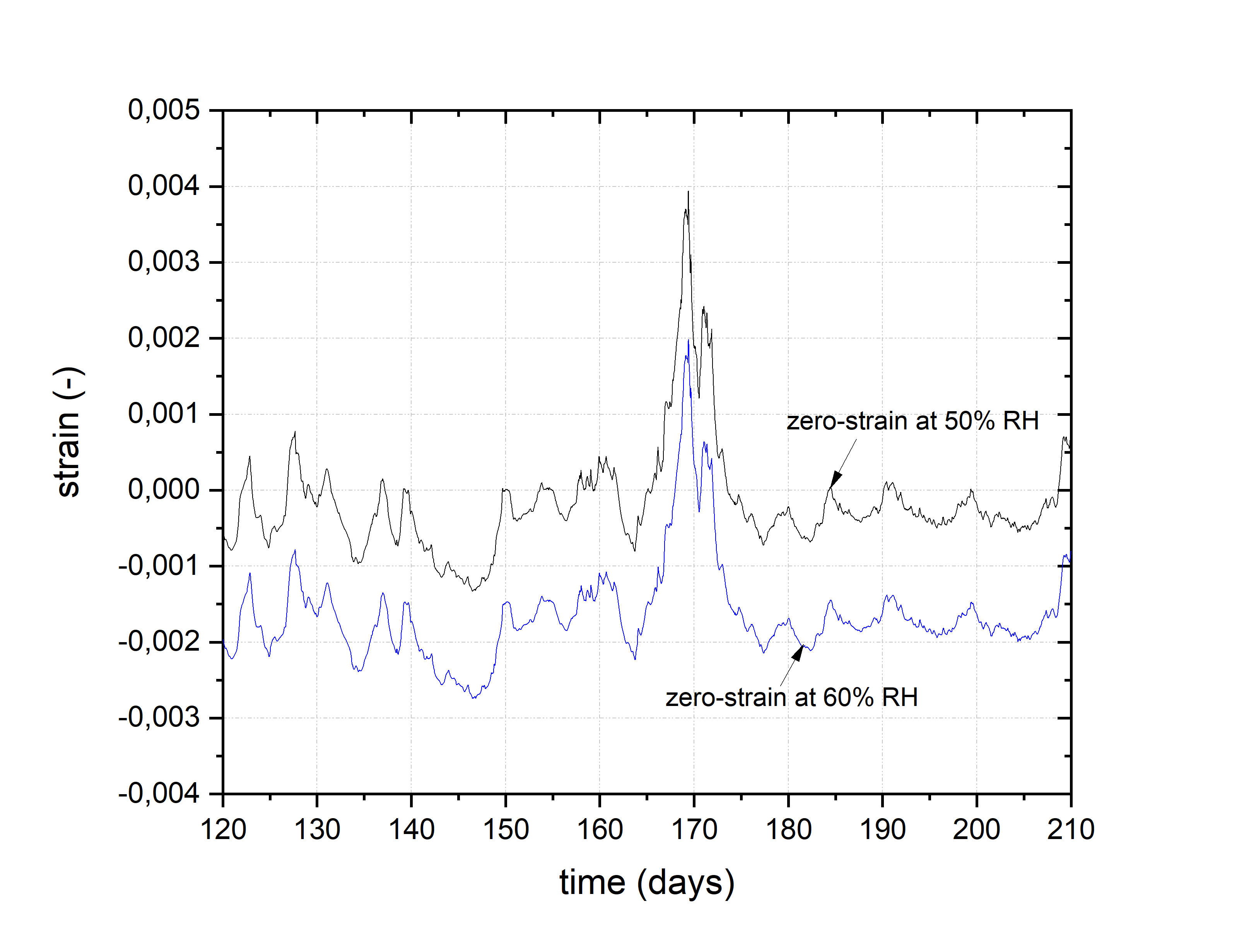
The next necessary operation is the scaling of the amplitude of the strain history. This operation reflects the fact that the same RH cycle yields different elementary strain cycles depending on the zero strain RH level assumed, as illustrated in the figures below.

An elementary RH cycle of +/- 2% centred at 60%.

The amplitude of an elementary strain cycle – induced by the elementary RH cycle shown above – is lower in the case of zero-strain RH level at 60%, versus a zero-strain RH level at 50%.

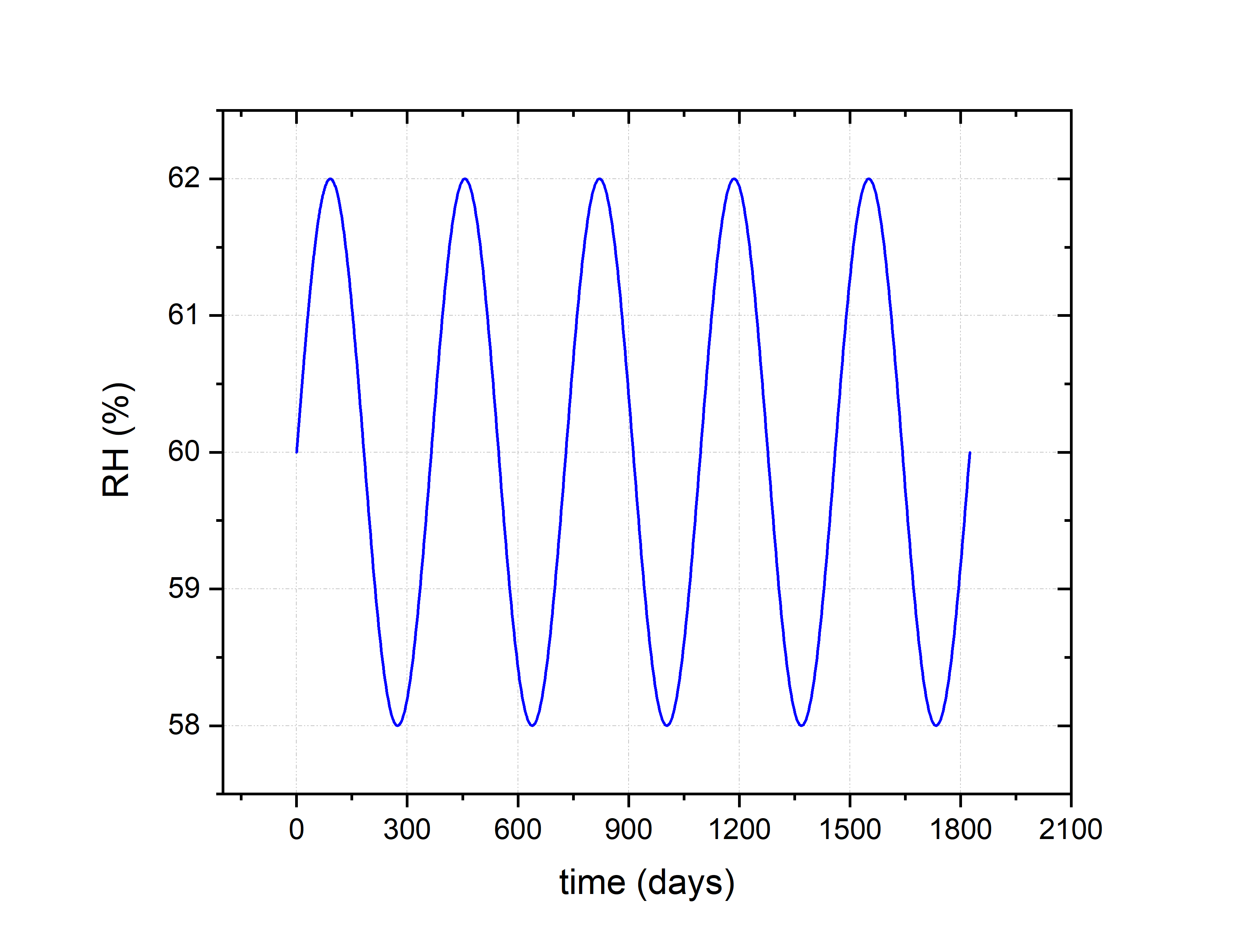
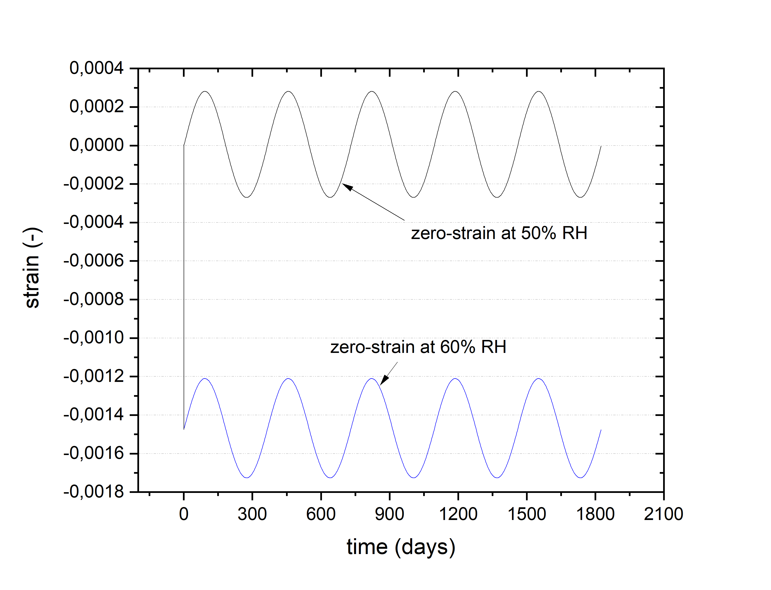
The scaling factors, which are multiplied by the strain histories in order to account for a selected zero-strain RH level, are pre-calculated in the software for systematically varied RH levels.

Step 5 – Calculating risk indices

The final step of the analysis is the risk assessment of physical damage by the user who selects a damage criterion. The criterion is based on a critical level of dimensional response bringing damage. Currently, strains at yield and at break are provided in the software as the damage criteria for wood and strain at failure for gessoes. Details are given in the respective criterion sections of the manual.

Validation of the model

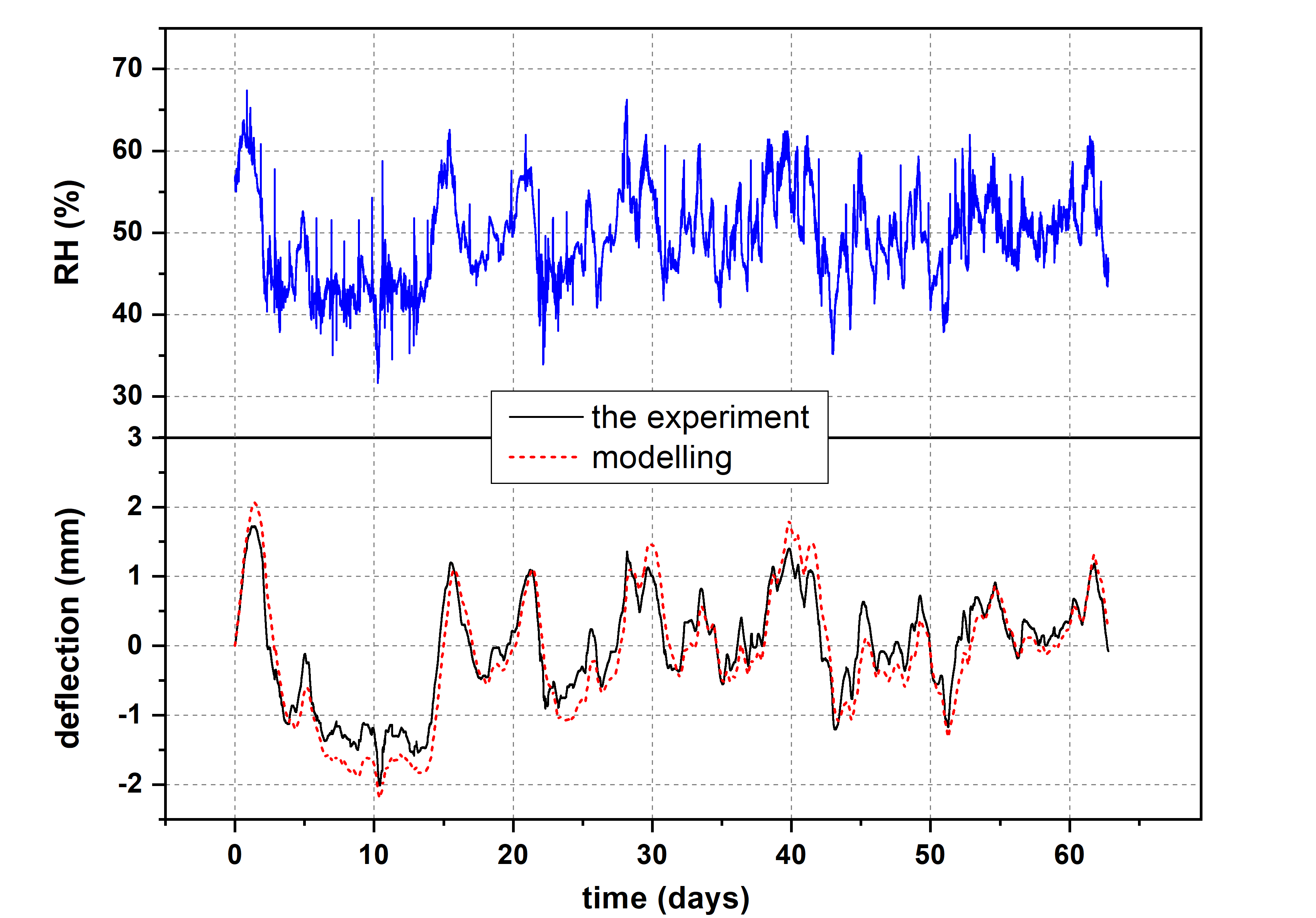
The finite element numerical simulation methods used in the tool were validated by comparison to experimental measurements. A 10 mm thick panel of lime wood covered with 0.5 mm layer of stiff gesso was exposed to real-world climate conditions in a gallery at the National Museum in Krakow. Water vapour transport was allowed through both faces. The deflection of this specimen, which imitates a panel painting, was measured using displacement sensors and modeled using numerical simulation. Comparison of the results depicted in the figure below shows a very good agreement between experiment and computation.

Experimental measurements compared to computational modeling results.

Further information

More information on the approach used in the software is contained in the publication:

A. Kupczak, M. Jędrychowski, Ł. Bratasz, M. Łukomski, R. Kozłowski, Processing relative humidity data using discrete Fourier transform to control strain in art objects . Strain, 55:e12311, 2019.

How the tool works – parchment

The rate of water vapour uptake or release by parchment is rapid compared to the duration of RH variations. The new equilibrium moisture content in the material is established after an RH change in less than one hour. Therefore, RH variations are translated by the software into the moisture related dimensional change (strain), by assuming that parchment reaches its full dimensional response at each instant of the variation.

The dimensional change isotherm demonstrates the relationship between moisture related strain and the RH at a given temperature and indicates the amount of swelling or shrinkage experienced by parchment based on an increase or decrease in RH. We have determined the dimensional change isotherms for several specimens of historical and contemporary parchments produced in a manner similar to the historical material. The measurements were performed in two perpendicular directions to account for possible effects from preferred collagen fibre orientations. Indeed, the data demonstrated a difference in the moisture-related dimensional change between the two directions. The contemporary parchment exhibited a larger moisture-related response compared to most historical materials, therefore it can be regarded as the worst-case material in terms of the climate-induced risks to parchment.

In the software, the scanning dimensional change isotherm of contemporary parchment in the direction of largest response was used to account for the effect of sorption hysteresis in parchment - see figure below. The scanning isotherm was obtained using the approach of Mualem [ref. 1]. The dimensional changes at RH intervals of 5% were calculated using the swelling - shrinkage path following the changes in RH 0% → 80% → 10% → 50% → 45% → 55% → 40% → 60% → etc.

Moisture related swelling and shrinkage of contemporary parchment at 24 ^oC.

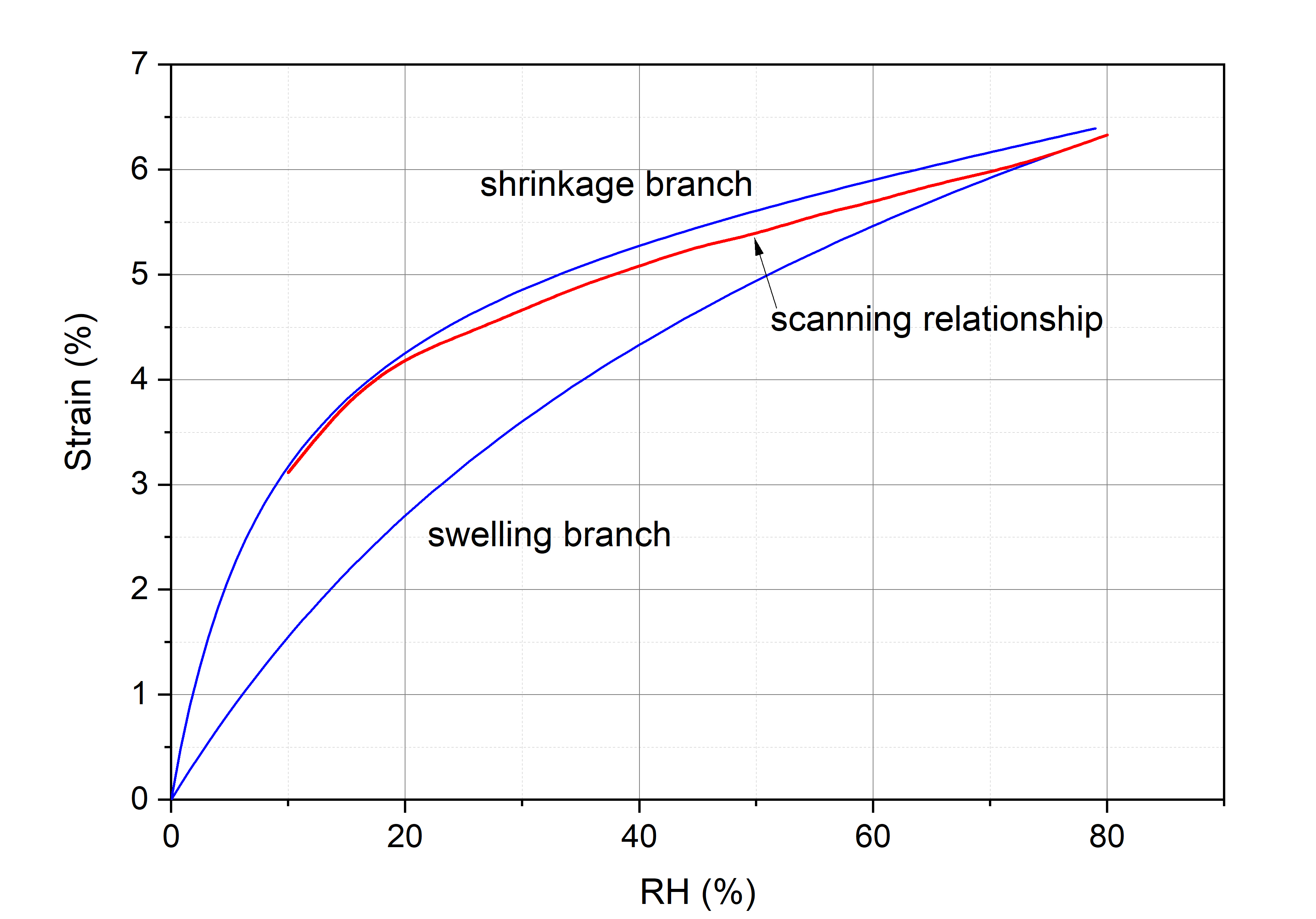
Fitting the three-parameter equation of the following form:

to the scanning dimensional change isotherm of parchment gave the values of the constants a, b and c shown in the table below

1. Y. Mualem, A conceptual model of hysteresis, Water Resources Res., 10, 514-520, 1974.

Further information

More information on the approach used in the software is contained in the publication:

L. Krzemień, A. Czyżewska, M. Soboń, R. Kozłowski, Ł. Bratasz, Risk of climate-induced damage in historic parchment, Heritage Science, 8:17, 2020.

The effect of cracks on strain in the pictorial layer

More information on the impact of crack patterns in panel paintings on the risk of new crack development is contained in three publications:

2. Ł. Bratasz, M.R. Vaziri Sereshk, Crack saturation as a mechanism of acclimatization of panel paintings to unstable environments, Studies in Conservation, 63:sup1, 22-7, 2018.

3. M.Y.A. Jamalabadi, N. Zabari, Ł. Bratasz, Three-dimensional numerical and experimental study of fracture saturation in panel paintings, Wood Science and Technology, 55,1555-76, 2021.

Development of craquelure patterns in paintings on panels, Heritage Science, 12:89, 2024.

Strain at which gesso cracks as the damage criteria for the gesso layer on an unrestrained wood panel

Gesso deforms when force is applied, and the stress-strain curves illustrate subsequent phases of the deformation by increasing stress. Strain is the change in length divided by the specimen’s original length, and stress is calculated by dividing the force (load) applied to the test specimen by its cross- sectional area. The final recorded point of the stress-strain curve is the strain at which gesso cracks. The mechanical properties of gesso depend on the strength of the collagen glue used, the ratio of the inert solid (the pigment) to the glue, and the ambient RH, as gesso undergoes a transition from the brittle to the ductile state with increasing RH.

The stress–strain curves for the gesso tested at various relative humidity values.

Elongation at which gesso cracks is approximately 0.002 for stiff and brittle gessoes in the low and middle range of RH, considered the worst- case conditions for gesso’s vulnerability to fracture, but increases by an order of magnitude with increasing RH.

Upon a decrease in RH, wood undergoes shrinkage, inducing compressive stress and negative strain in the gesso layer, whereas upon an increase in RH, wood undergoes swelling, inducing tensile stress and positive strain in the gesso layer. The HERIe software uses the strain threshold of 0.002 to calculate the risk index for a given strain versus time history: strain is calculated as a change in the length of the interface between the gesso layer and the wood support divided by the length of this interface at the assumed zero- strain RH level (see ‘How the tool works – wooden panels’).

Water vapour transport through faces of a painted/decorated panel

Free water vapour transport through only one face of a panel simulates the extreme barrier effect of pictorial or decorative layers comprising oil paints, gilding and/or varnishes. In this configuration, the panels initially experience moisture change and dimensional response at the bare wood surface opposite to the painted/decorated face. Only when the duration of an RH variation increases, does moisture content become uniform across the panel and the effect of differences in the moisture permeability of the two faces gradually vanishes.

Free water vapour transport through both faces of a panel simulates a bare wooden panel or the minor barrier effects offered by an egg or glue tempera on a gesso ground layer. In this configuration, the response time of panels to RH variations is shorter as the panels experience moisture change through two faces.

Detailed information on the water vapour permeability of pictorial layers on wood, replicating materials and techniques traditionally used in Europe is provided in:

Allegretti, O. and Raffaelli, F. "Barrier effect to water vapour of early European painting materials on wood panels"Studies in Conservation, 53, 187–197, 2008

Strains at which gesso irreversibly deforms or breaks as the damage criteria for the gesso layer on an unrestrained wood panel scenario

Marion Mecklenburg and his collaborators at the Smithsonian Institution proposed that the two critical values by which the risk of damage should be assessed are the strains at which a material irreversibly deforms or breaks (see ref. 1 for the detailed discussion).

Gesso deforms when force is applied and the stress–strain curves illustrate subsequent phases of the deformation initiated by increasing stress. Strain is the change in length divided by the specimen original length and stress is calculated by dividing the force (load) applied to the test specimen by its cross-sectional area. The strain that can be recovered immediately on the release of the stress is termed the elastic response. When strain reaches the upper limit of the elastic range, a non-recoverable plastic deformation begins. It is known to occur near, or above, the point where the curve begins to deviate significantly from a straight line. The final recorded point of the stress–strain curve is the strain at which gesso breaks via fracture.

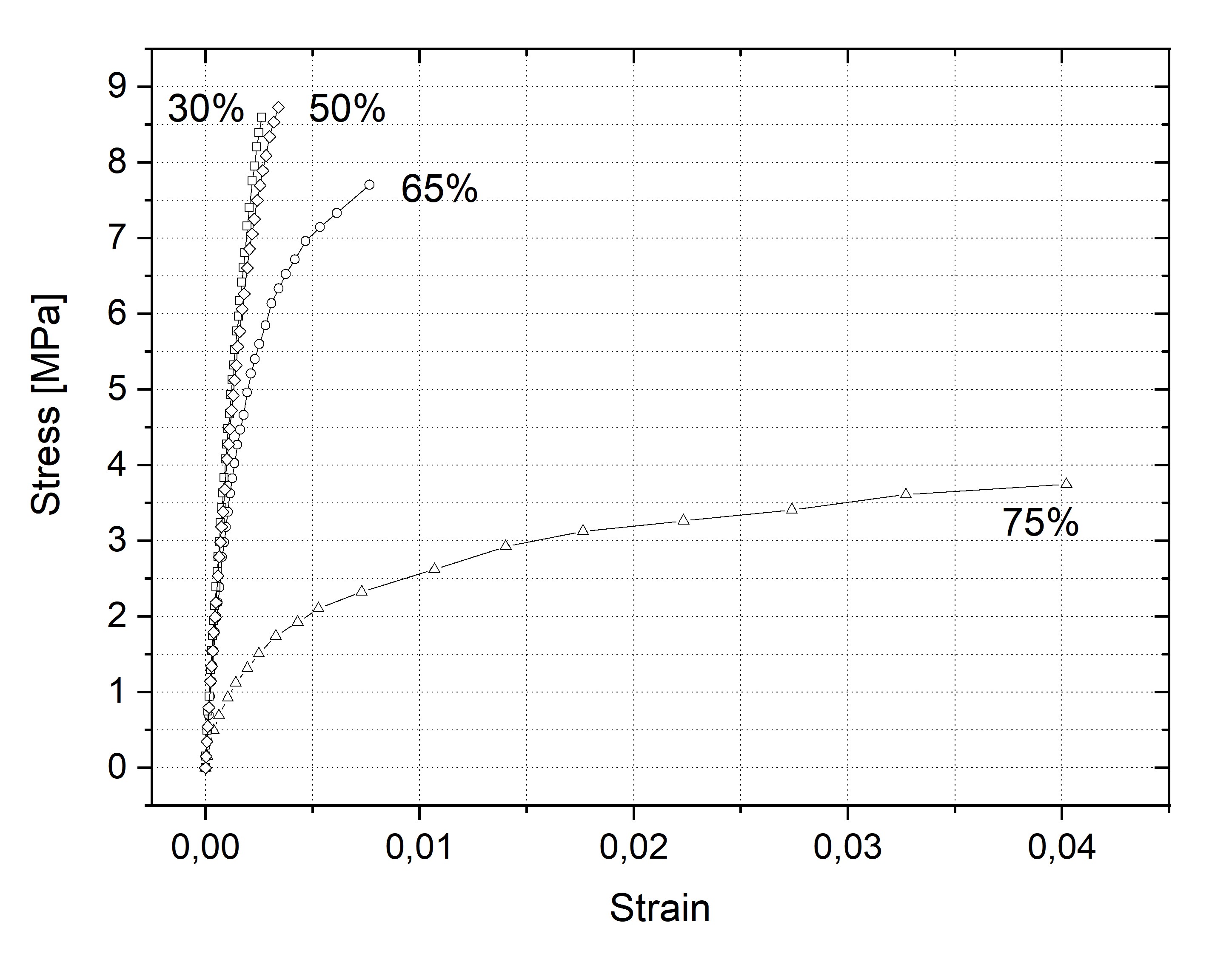
The stress–strain curves for the gesso tested at various relative humidity values.

Upon decrease in RH wood undergoes shrinkage which induces compressive stress and negative strain in the gesso layer, whereas upon increase in RH wood undergoes swelling which induces tensile stress and positive strain in the gesso layer.

The mechanical properties of gesso depend on the strength of the collagen glue used, the ratio of the inert solid, ‘the pigment’, to the glue and ambient RH as the gesso undergoes transition from the brittle to the ductile state with increasing RH. Strains at which stiff and brittle gessoes irreversibly deform or break are considered the worst case conditions for the gesso’s vulnerability to damage. These two critical strains, determined experimentally for the RH mid-range to be 0.002 and 0.004, respectively (refs. 1 and 2) are used to calculate the risk index for a given strain history – strain is calculated as a change in the length of the interface between the gesso layer and the wood support, divided by the length of this interface at the assumed zero-strain RH level (see ‘How the tool works – wooden panels’):

• when the absolute maximum magnitude of strain experienced by the gesso layer (in compression or tension) does not exceed 0.002, the risk index is 0
• when the absolute maximum magnitude of strain experienced by the gesso layer (in compression or tension) exceeds 0.004, or the double strain at which gesso cracks, the risk index is 1,
• for compressive or tensile strain magnitudes between 0.002 and 0.004, the risk index increases linearly between 0 and 1

Notice: the user can calculate his or her own risk indices by reading maximum strains from the strain histories calculated by the tool and using higher critical strains than those proposed above as the most conservative, worst case scenario. For example, critical strains of 0.005 and 0.01 respectively, were determined for gessoes investigated in Ref. 3.

1. Mecklenburg, M.F., Tumosa, C.S. and Erhardt, D. 1998. Structural Response of Painted Wood Surfaces to Changes in Ambient Relative Humidity. In: V. Dorge & F.C. Howlett, eds. Painted Wood: History and Conservation. Los Angeles: The Getty Conservation Institute, pp. 464–83.

2. Rachwał, B., Bratasz, Ł, Krzemień, L., Łukomski, M. & Kozłowski, R. 2012. Fatigue damage of the gesso layer in panel paintings subjected to changing climate conditions, Strain, 48: 474-481.

3. Mecklenburg, M. 2011. Determining the Acceptable Ranges of Relative Humidity and Temperature in Museums and Galleries. Report of Museum Conservation Institute, the Smithsonian Institution. Available at https://www.si.edu/mci/english/learn_more/publications/reports.html.

Strains at which wood irreversibly deforms or breaks as the damage criteria for a fully restrained wooden panel

Marion Mecklenburg and his collaborators at the Smithsonian Institution proposed that the two critical values by which the risk of damage should be assessed are the strains at which a material irreversibly deforms or breaks (see ref. 1 for the detailed discussion).

Wood deforms when force is applied and the stress–strain curves illustrate the subsequent phases of the deformation initiated by increasing stress. Strain is the change in length divided by the specimen original length and stress is calculated by dividing the force (load) applied to the test specimen by its cross-sectional area. The strain that can be recovered immediately on the release of the stress is termed the elastic response. When strain reaches the upper limit of the elastic range, a non-recoverable plastic deformation begins. It is known to occur near, or above, the point where the curve begins to deviate significantly from a straight line. The final recorded point of the stress–strain curve is the strain at which wood breaks via fracture.

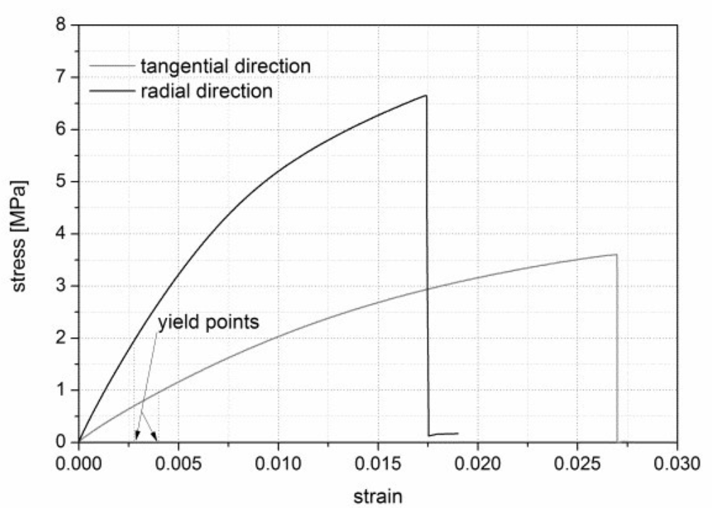
The stress–strain curves for lime wood at relative humidity of 50%. The yield strains are indicated by the arrows. These are considerably lower than the strains required to cause the wood to break.

When wood is restrained from movement and desiccated upon fall in ambient RH, it experiences an increase in tensile strain, as the material effectively undergoes free shrinkage and is ‘stretched’ back to its original restrained length. Similarly, if wood is restrained from movement and humidified, it experiences an increase in compressive strain, as effectively the material undergoes free swelling and is ‘compressed’ back to its original restrained length. Restraint may result from rigid construction restricting movement, or by assembling wood elements with different orientations of their fibre directions. Wood can also experience internal restraint as the moisture diffusion is not instantaneous. An uneven moisture change will induce an uneven dimensional response when the outer face of the wood responds more quickly than the interior to variations in ambient RH. Uneven dimensional response to moisture flow in opposite faces of decorated panels due to a lower permeability of the painted/gilded face is another cause of restraint.

The critical strains perpendicular to grain, at which wood deforms irreversibly or breaks, are generally around 0.005 and 0.02 respectively, at the RH mid-range (ref. 1). The risk index for a given strain history is calculated in the following way:

• when the absolute maximum magnitude of strain experienced by a fully restrained wooden element (in compression or tension) does not exceed 0.005, the risk index is 0,
• when the absolute maximum magnitude of strain experienced by fully restrained wooden element (in compression or tension) exceeds 0.02, the risk index is 1,
• for compressive or tensile strain magnitudes between 0.005 and 0.02, the risk index increases linearly between 0 and 1.

Notice: the user can calculate his or her own risk indices by reading maximum strains from the strain histories calculated by the tool and using other critical strains than those proposed above.

1. Mecklenburg, M.F., Tumosa, C.S. and Erhardt, D. 1998. Structural Response of Painted Wood Surfaces to Changes in Ambient Relative Humidity. In: V. Dorge & F.C. Howlett, eds. Painted Wood: History and Conservation. Los Angeles: The Getty Conservation Institute, pp. 464–83.

Permanent curling and fracture on drying as damage criteria for restrained parchment

As the result of the collagen moisture-related dimensional response, parchment sheets shrink as they lose moisture and swell when they gain moisture, and they experience stress when restraint is placed on their dimensional response. Restraint may result from binding parchment sheets into a book block, attaching parchment with glue to rigid substrates as wooden book covers, or mounting a parchment sheet into a rigid housing (matting). Restrained swelling of parchment causes the material to curl whereas restrained shrinkage can additionally lead to physical failure.

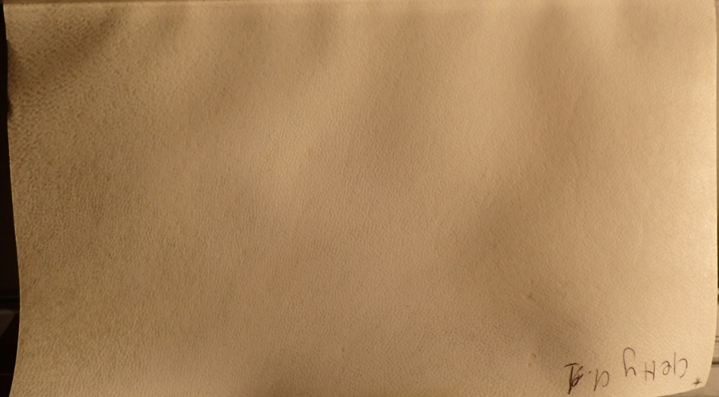
We have measured the permanent curling of parchment subjected to RH changes of increasing amplitudes. One edge of a flat even-surface parchment specimen stabilized at 50% RH was restrained in metal clamps. Then, the specimen was exposed to a given RH level and returned to 50% RH again. Sufficient exposure times were determined experimentally so that maximum curling was attained at RH levels different from 50% RH. Similarly, the potential for recovery of reversible curling was determined during the stabilization steps when the specimens were returned to 50% RH and before permanent curling was induced by progressively larger changes (see the photograph below). The curling was measured by scanning the specimen surface with the use of a laser profilometer. Then the local curvature in the direction parallel to the clamps was calculated for all scanned points.

An example of parchment’s permanent curling due to cycling RH with a restraint placed at the top of the specimen.

The distribution of local curvatures has a characteristic Gaussian shape peaking around zero curvature with positive and negative deviations from a flat plane increasing with the increased distortion. The acquired data were smoothed and a synthetic parameter characterizing parchment curling was calculated as the standard deviation of local curvatures. The increase in irreversible curling produced by variations in RH is shown in the figure below. We selected three thresholds for degrees of curling – insignificant, visible and significant to represent the risk indices. They are marked with green, yellow and orange in the figure. Different stakeholder groups such as the general public, curators, and conservators may have varying opinions on how to determine the quantitative loss of aesthetic/display value of parchment objects resulting from increased curling.

Curling of contemporary parchment specimens after they were exposed to more humid (triangles) or arid (squares) conditions and then stabilized back at 50% RH.

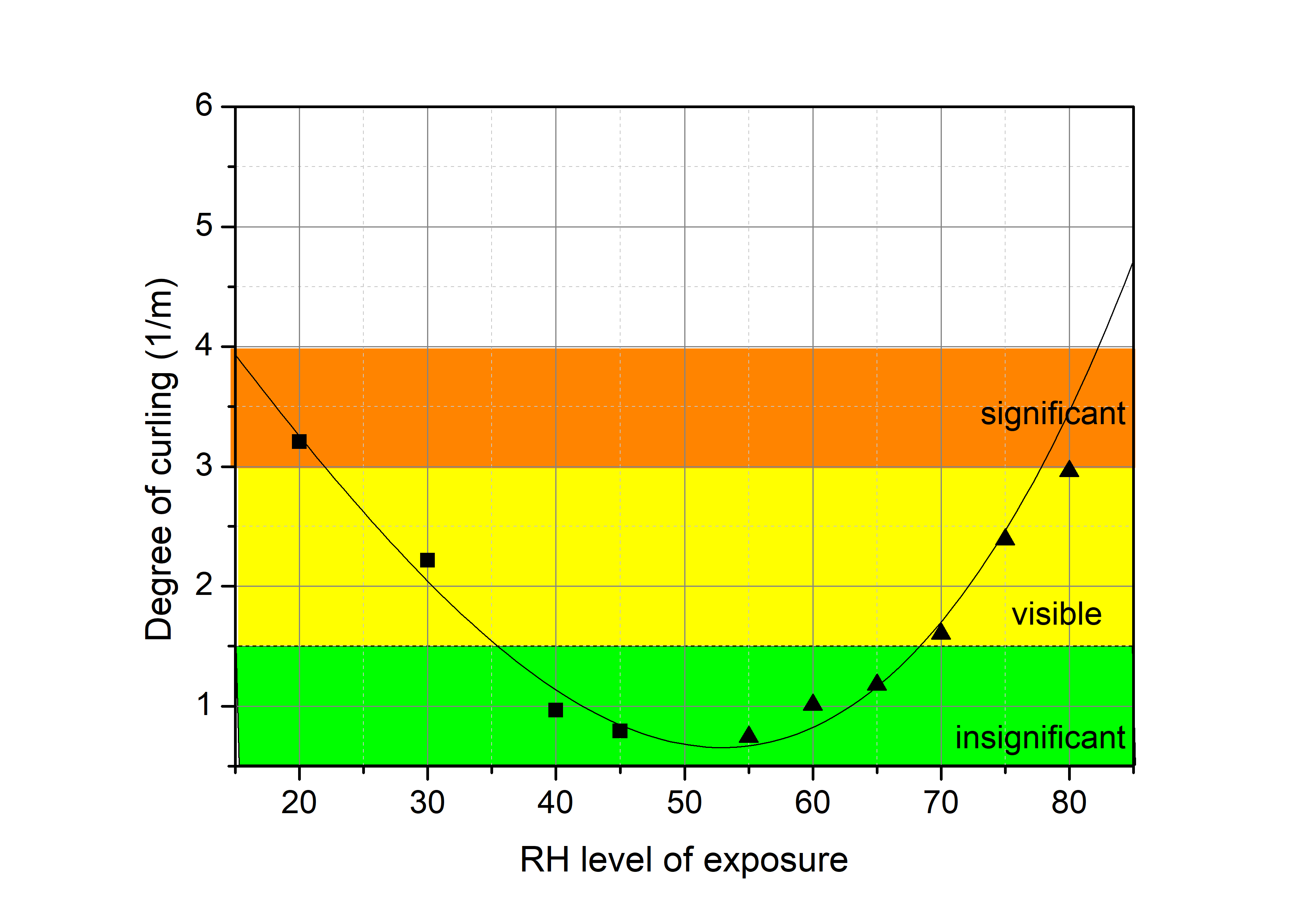
The following relationship between the degree of permanent curling and RH was obtained by fitting a third-order polynomial to the measurements:

\begin{equation} Degree\: of\: curling=0.13638\cdot RH-6.08366\cdot 10^{-4}\cdot RH^{2}+2.389\cdot 10^{-5}\cdot RH^{3} \quad (1/m) \end{equation}

The risk index for a given RH versus time history is calculated in the following way:

• when the maximum degree of permanent curling experienced by a restrained parchment sheet (on shrinkage or swelling) does not exceed 1.5 1/m, the risk index is 0,
• when the maximum degree of permanent curling experienced by a restrained parchment sheet (on shrinkage or swelling) is between 1.5 and 3 1/m, the risk index increases linearly between 0 and 1.

The proposed climate-induced risk is based on permanent curling of a flat, even-surface parchment sheet. Historical parchment documents, generally demonstrating considerable curling engendered by uncontrolled storage conditions in the past, are not vulnerable to further distortion when subjected to variations in RH even of considerable magnitude.

Further, the risk index for a given strain versus time history is assumed to be 1 when shrinkage strain experienced by a fully restrained parchment sheet exceeds 0.025 as we have determined that the risk of parchment fracturing above such strain increases.

Parameters for wood species and gessoes used in the modelling

Finite element numerical simulation used to create the software’s databases of elementary strain cycles solves the diffusion equation where the gradient of water vapour pressure is the driving force for the flow of moisture through the object. Then, the software calculates the dimensional response (strain field) across the object, based on the moisture-related (adsorption/desorption and swelling/shrinkage) and mechanical properties of materials. Below, information is provided on all parameters for wood species and gessoes used for strain modelling in the software. The parameters come from our own measurements or relevant publications which are referenced.

Water vapour sorption isotherms

The sorption isotherm is the relationship between the equilibrium moisture content M and the relative humidity RH and is key to determining the amount of water vapour that a material can store at a given RH. Sorption isotherms for three species of wood – lime, oak and poplar [ref. 1] as well as for typical gesso of the pigment-volume concentration (PVC) of 92% [ref. 2] are used in the modelling. PVC is defined as \begin{equation} PVC = \frac{P}{P + B}*100 % \end{equation} where P and B are volumes of chalk (the pigment) and the dried glue binder, respectively. The three-parameter Guggenheim-Anderson-de Boer (GAB) sorption equation of the following form:

\begin{equation} M(RH,T= \mbox{const.}) = \frac{V \cdot c \cdot k \cdot RH /100 }{(1-k \cdot RH/100) \cdot (1+(c-1)\cdot k \cdot RH/100 )} \end{equation}

was fitted to the sorption data, which gave the values of the GAB constants V, c and k given in Table 1.

In modeling, the scanning sorption isotherm for each wood species is used to account for the effect of sorption hysteresis in wood (see figure below). The scanning isotherms were calculated at RH intervals of 5% in the RH range of 5-95% using the approach of Mualem [ref. 3] and the adsorption - desorption path following this pattern of changes in RH: 0% → 94% → 20% → 50% → 45% → 55% → 40% → 60% → etc.

Adsorption and desorption of water vapour for lime wood at 24^oC: the re-adsorption path following the change in RH from 20 to 94% predicted by modelling (dotted line) and measured experimentally (•).

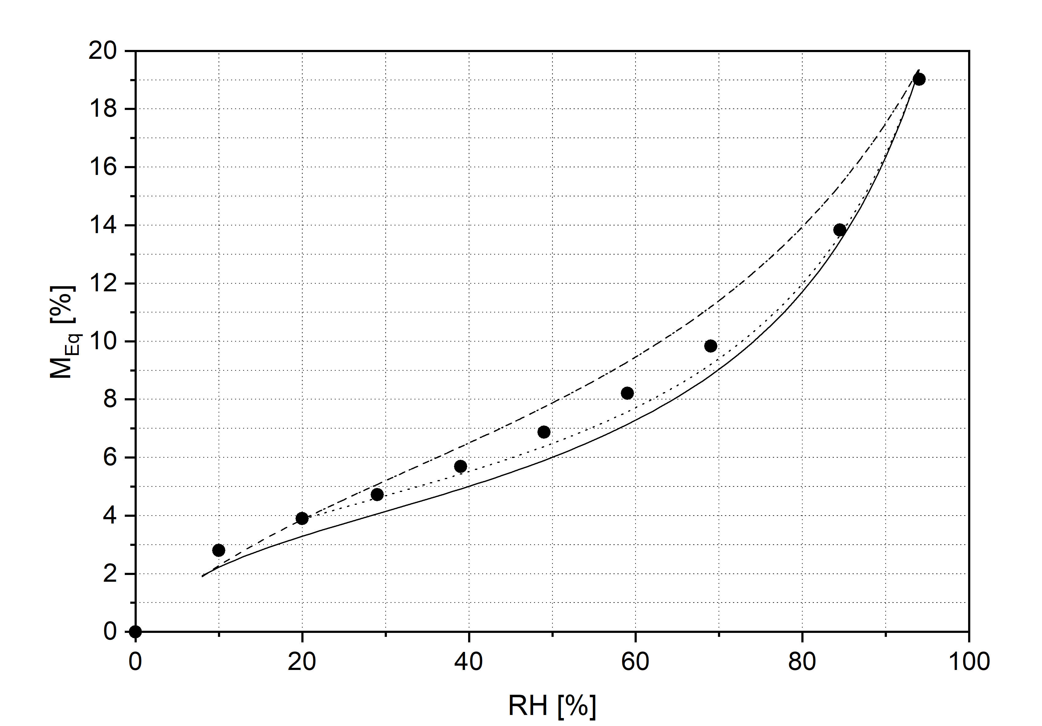
Fifth degree polynomial functions fitted to the scanning isotherms are given in Table 2.

Water vapour diffusivity

A general curve describing the relationship between water vapour diffusivity in wood, D, and RH proposed by Time [ref. 2] with a temperature modification factor proposed by Simpson [ref. 5] was used in the model: \begin{equation} D (T,RH) = 1.44 \cdot 10^{-7} \cdot RH^{-1.8449} \cdot exp(\frac{-5280}{T}) \end{equation} where \( D \) is in kg/msPa and \( T \) is temperature in K. The general relationship was verified to adequately capture the variability of these parameters inherent to various species and anatomical directions in wood.

No measureable barrier effect to water vapour diffusion due to the gesso layer could be observed when compared to the results for bare wood [ref. 3]. Consequently, for the purpose of this model, water vapour diffusivity in the gesso is simply treated as 20 times greater than that of wood.

External mass transfer coefficient

Water vapour passing through the wood surface encounters a barrier in the form of an air layer adjacent to the surface. This resistance is described by the external mass transfer coefficient in kg/m²sPa which tells how many kilograms of water vapour pass through 1m² of the surface during one second under the 1Pa gradient of the water vapour pressure. The value of this parameter depends on the intensity of air motion in a specific environment. The parameter used in this model is 3·10^-8 kg/m²sPa and reflects environments with considerable air motion typical of museum galleries and the interiors of historical buildings.

Moisture related dimensional response

The moisture-related strain (ε) of individual wood species – swelling or shrinkage in the radial and tangential anatomical directions – is expressed as a sigmoid function of moisture content M:

where ε is the strain related to the initial dry length. Parameters of the function obtained from the regression of the experimental data [ref. 6] are given in Table 2.

In turn, the moisture related dimensional change coefficients for the gessoes are expressed per change in RH and are given in Table 3.

Mechanical properties - elasticity moduli, Poisson’s coefficients, shear moduli

Mechanical properties of wood and gesso, necessary to model their stress and strain fields are gathered in this section.

Elasticity moduli for wood species in their two anatomical directions, radial and tangential, along with the same parameter for the gessoes, as a function of RH, are given in Table 4

Poisson’s ratios for wood \( {\large \nu_{TR}} \) corresponding to a contraction in the R direction when the tension is applied along the T direction are given in Table 5.

As wood is an orthotropic material,\( {\large \nu_{RT}} \) was calculated according to the equation below:

Poisson’s ratio of gesso is 0.2.

Shear moduli

The shear modulus of wood is calculated as a function of its elasticity modulus and Poisson’s ratio by the following formula:

Density

References

1. Ł. Bratasz, A. Kozłowska, R. Kozłowski, Analysis of water adsorption by wood using the Guggenheim-Anderson-de Boer equation, European Journal of Wood and Wood Products, 70, 445-451, 2012.

2. B. Rachwał, Ł. Bratasz, L. Krzemień, M. Łukomski, R. Kozłowski, Fatigue damage of the gesso layer in panel paintings subjected to changing climate conditions, Strain, 48, 474-481, 2012.

3. Y. Mualem, A conceptual model of hysteresis, Water Resources Res., 10, 514-520, 1974.

4. B. Time, Hygroscopic moisture transport in wood, published by the Norwegian University of Science and Technology, Department of Building and Construction Engineering, 1998, pp. 128-130.

5. W. T. Simpson, Determination and use of mosture diffusion coefficient to characterize drying of northern red oak (Quercus-rubra), Wood Science and Technology, 27, 409-420, 1993.

6. Ł. Bratasz, R. Kozłowski, A. Kozłowska, B. Rachwał, Sorption of moisture and dimensional change of wood species used in historic objects, in Wood Science for Conservation of Cutural Heritage, Braga, 2008: Firenze University Press, pp. 14-16.

7. D. W. Green, J. E. Winandy, D. E. Kretschmann, Wood Handbook, Wood as an Engineering Material. Madison: Forest Products Society, 1999.

8. G. van Gerven, B. Ankersmit, P. van Duin, A. Jorissen, H. Schellen, A controlled method to flatten warped wooden panels, Studies in Conservation, 61, 125-135, 2016.

9. M. Merela, K. Cufar, Mechanical properties of sapwood versus heartwood, in three different oak species, Drvna Industrija, 64, 323-334, 2013.

10. P. Mazzanti, M. Togni, L. Uzielli, Drying shrinkage and mechanical properties of poplar wood (Populus alba L.) across the grain, Journal of Cultural Heritage, 13, S85-S89, 2012.

11. B. Rachwał, Ł. Bratasz, M. Łukomski, R. Kozłowski, Response of wood supports in panel paintings subjected to changing climate conditions, Strain, 48, 357-444, 2012.